How to Use the Filter and Sort Data Function in Microsoft Excel

Things to Note About Using the Filter and Sort Function
The Filter function allows you to extract data from a data set that fits your criteria. It is great for data analysis. You can use the Filter function with a single criteria or multiple criteria. The Filter function looks like the below:
=FILTER(array,include,[if_empty])
- Array (required): This refers to the range or data set to be filtered. It is usually a table within the Excel worksheet but can also be a row or column with values.
- Include (required): This specifies the data to be extracted
- If empty (optional): This is the result to be shown if no items exist for the criteria specified.
The Sort function can also be used to sort the content of a range or array in the order you specify. The Sort function looks like the below:
=SORT(array,[sort_index],[sort_order],[by_col])
- Array (required): This refers to the range or data set to be filtered. In most cases, it is usually a table within the Excel worksheet, but it can also be a row or column with values.
- sort_index (optional): This specifies the number of the row or column to sort by
- sort_order (optional): This specifies the number for the desired sorting order. To sort by ascending order, use 1; for descending order, use -1.
- by_col (optional): This specifies the desired sort direction by row or column.
How to Use the Filter Function
When you filter, your functions depend on whether you need a single or multiple criteria in your filters. We explore both below.
Single Criteria
In a situation where you need to filter data based on just one criteria, here’s how you can do so with the Filter function:
Step 1: Open the Microsoft Excel app or workbook.
Step 2: Type the function below and the Tab button in an empty cell.
=FILTER

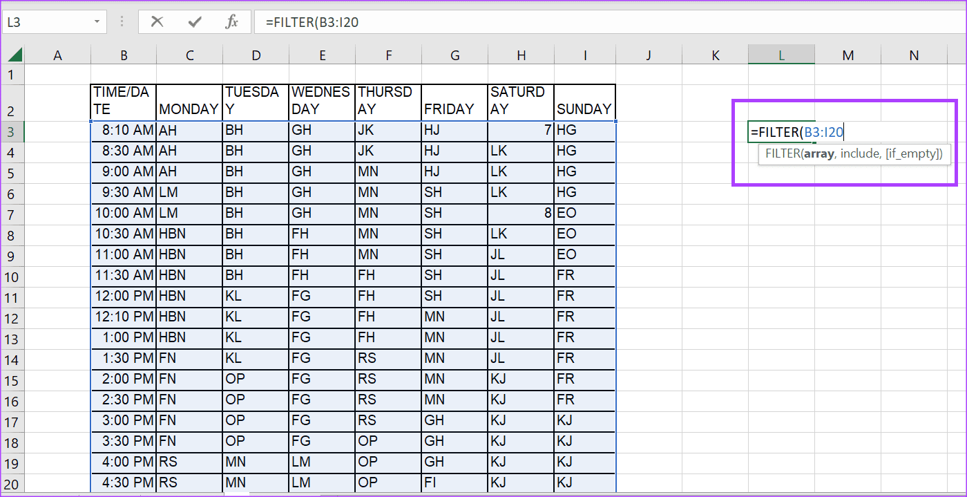
Step 3: Select the array with the dataset you would like to filter. In our example, we are selecting cells B3 to I20, which contains the information we want to filter for. So, we have:
=FILTER(B3:I20,
Step 4: Enter the criteria you want to filter in the include section. In our example, we are filtering for value HJ within column G. So, we have:
=FILTER(B3:I20,G3:G20=”HJ”,
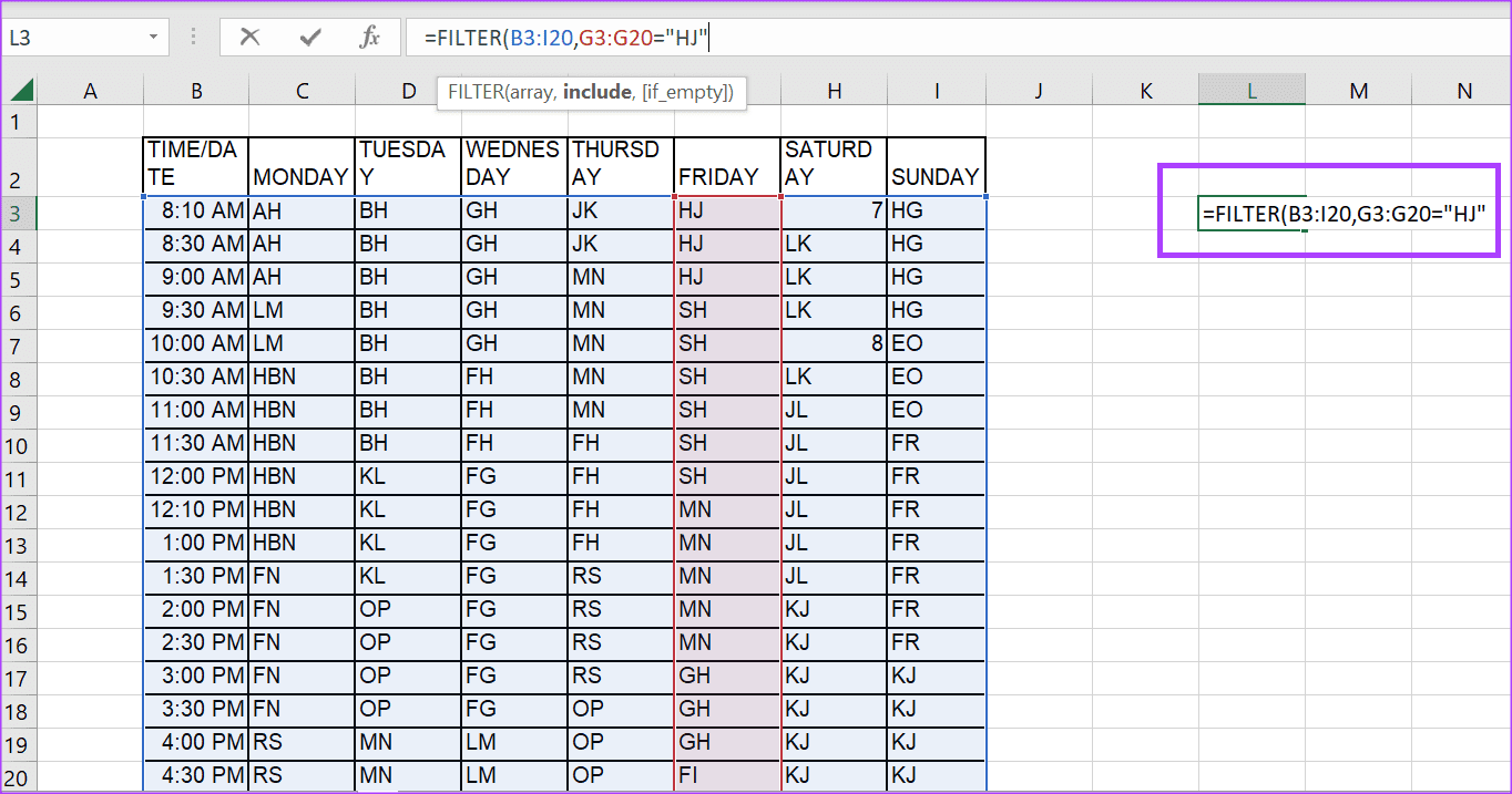
Note: You can directly include the criteria you are filtering for in the formula like we have done above or type it in a cell and refer to it within the formula. Typing it in a separate cell ensures you only have to edit that one cell when changing the criteria. However, if you write it directly in the formula, you must edit it to update the criteria.
Step 5: Enter the value you want Excel to return if any value in the array does not meet your criteria. In our example, we want Excel to return N/A if our criteria are unmet. You can also ask Excel to return an empty string using “”. So, we have:
=FILTER(B3:I20,G3:G20="HJ","N/A") or =FILTER(B3:I20,G3:G20="HJ","")
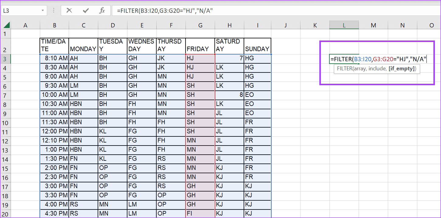
Step 6: Tap Enter for Excel to return results based on your set criteria.
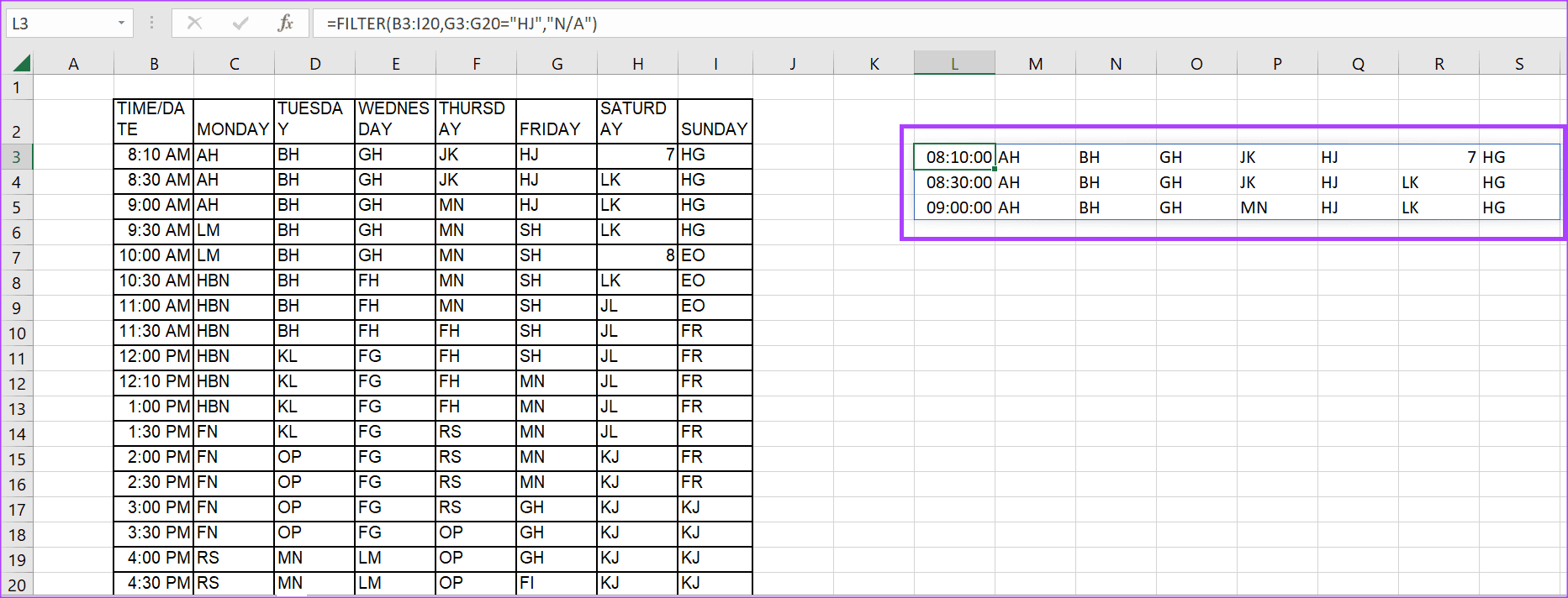
Multiple Criteria
You can combine multiple criteria to filter a dataset using the Filter function. To combine multiple criteria, you can use different Excel operators, such as (*) for AND with the Function formula. Here’s how to do so.
Step 1: Type the function below and the Tab button in an empty cell.
=FILTER
Step 2: Select the array with the dataset you want to filter. In our example, we select cells B3 to I20, which contains the information we want to filter. So, we have:
=FILTER(B3:I20,

Step 3: Enter the criteria you want to filter in the include section. In our example, we filter for value HJ within column G, and in column C, we filter for HBN. So, we have:
=FILTER(B3:I20,(G3:G20="HJ")*(C3:C20="HBN")
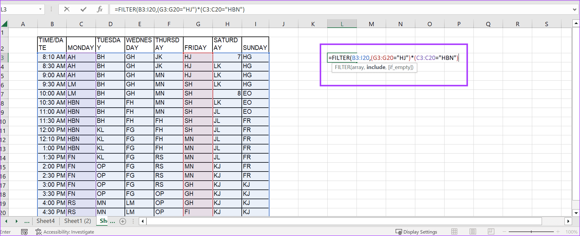
Step 4: Enter the value you want Excel to return if any value in the array does not meet your criteria. In our example, we want Excel to return N/A if our criteria are unmet.
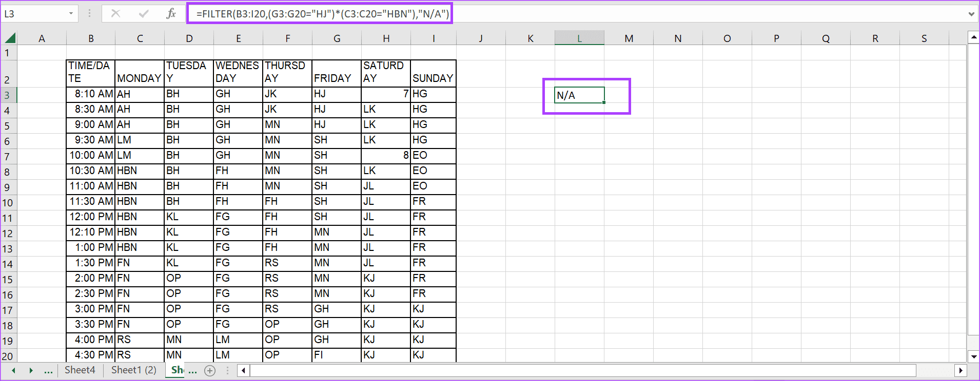
=FILTER(B3:I20,(G3:G20="HJ")*(C3:C20="HBN"),"N/A")
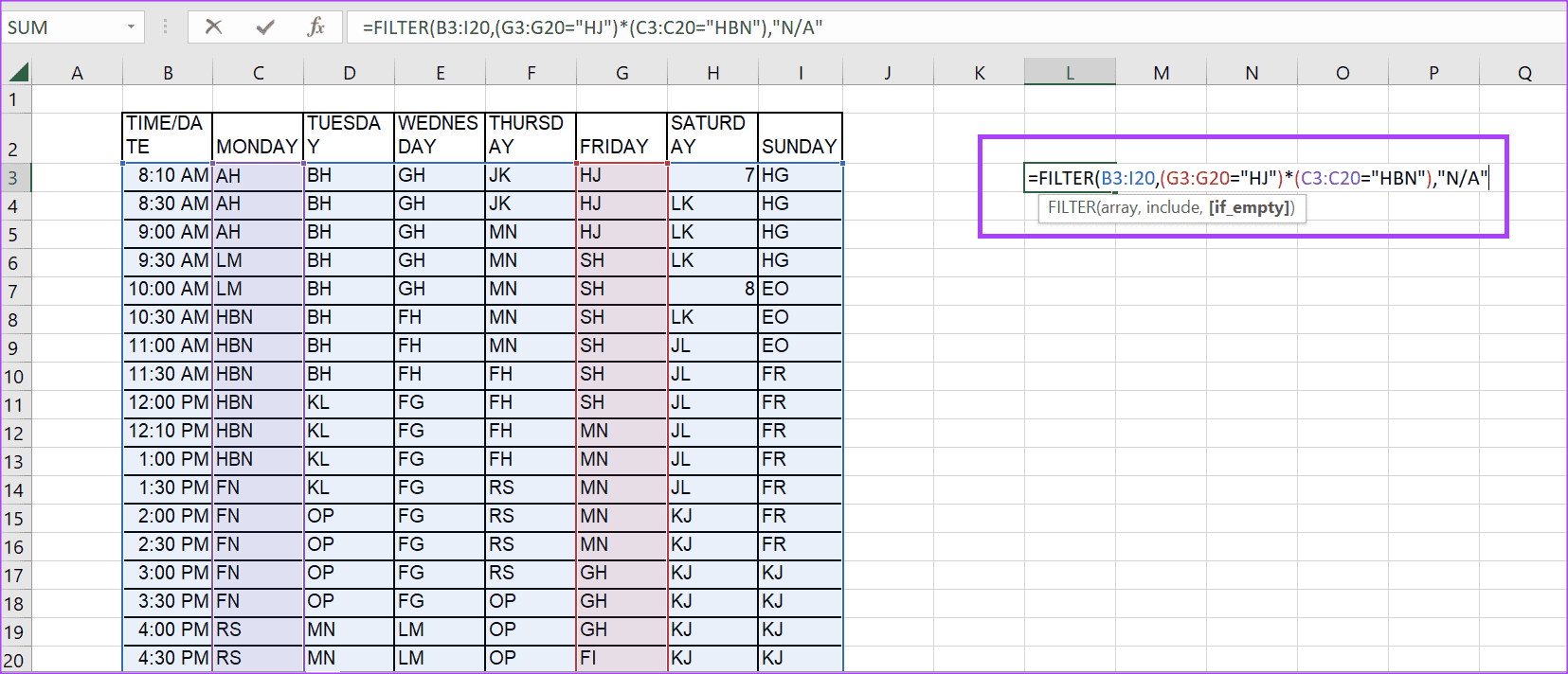
Step 5: Tap Enter for Excel to return results based on your set criteria.
How to Use the Sort Function
When you sort, your functions depend on whether you need to sort through a single or multiple columns. We explore both below.
Single Column
Step 1: In an empty cell, type the function below and tap the Tab button.
=SORT
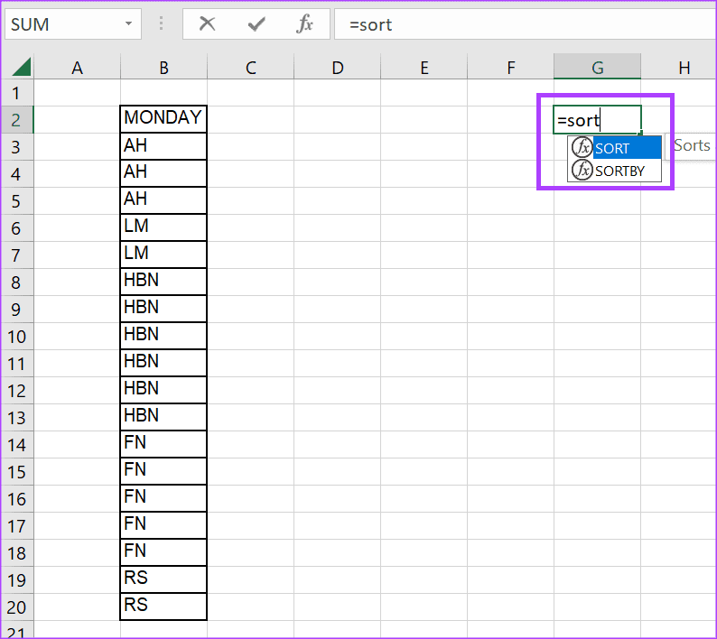
Step 2: Select the array with the dataset you want to sort. In our example, we select cells C3 to C20, which contain the information we want to sort. So, we have:
=SORT(B3:B20,
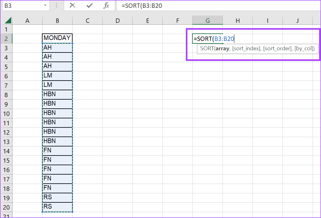
Step 3: Enter the row or column number to sort by. In our example, we only have one column. So, we have:
=SORT(B3:B20,1
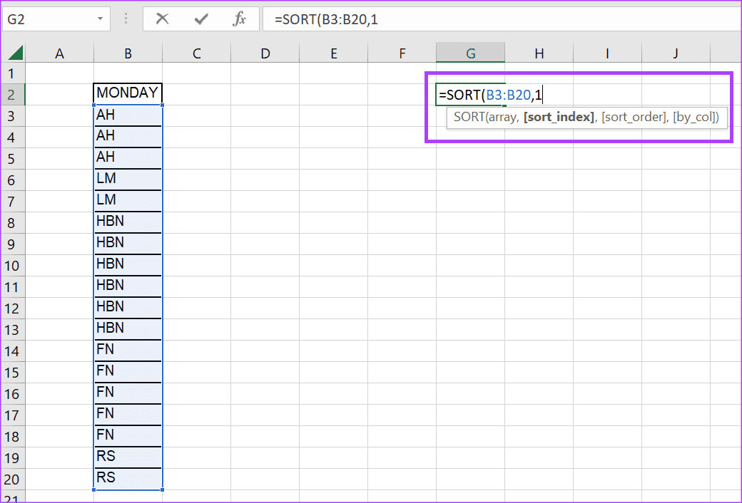
Step 4: Enter the order by which you want the data sorted. In our example, we are sorting in ascending order. So, we have:
=SORT(B3:B20,1,1)
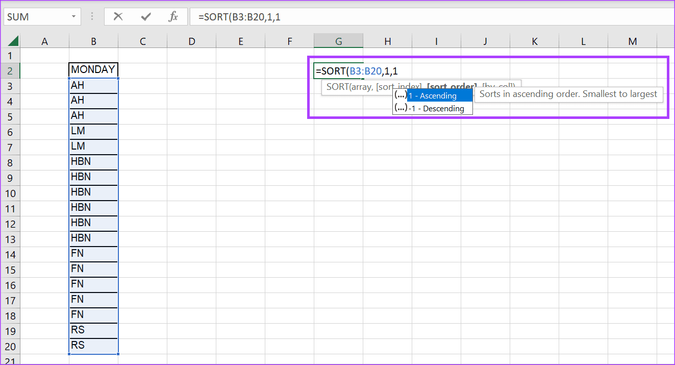
Step 5: Tap Enter for Excel to return results based on your sort criteria.
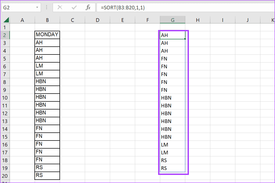
Multiple Columns
If you need to organize your data more comprehensively, you may need to sort it by multiple columns. Below is how to do this.
Step 1: In an empty cell, type the function below and tap the Tab button.
=SORT
Step 2: Pick your array with the sort dataset. To sort through multiple columns, we are using a wider array. Below, we select cells B3 to D20, So, we have:
=SORT(B3:D20,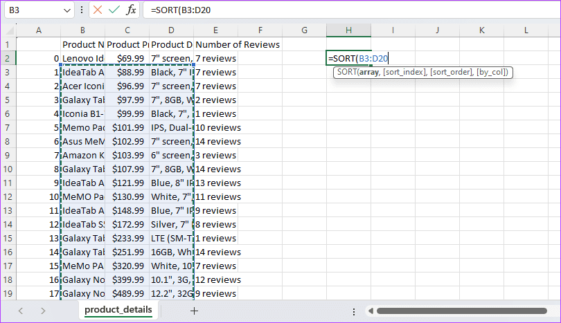
Step 3: Enter the column number to sort by. This corresponds to the position of the column within the selected array. So, if sorting by the second column in your range, your column number is 2. So, we have:
=SORT(B3:D20,2
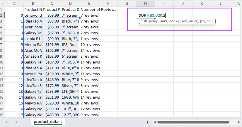
Step 4: Enter the order by which you want the data sorted. In our example, we are sorting in ascending order. So, we have:
=SORT(B3:D20,2,1
Step 5: Optionally, to include additional columns, add the SORTBY function nested within your SORT Function. So, to sort by the third column in descending order after sorting by the second column, include:
,SORTBY(B3:D20,D3:D20,-1))
Step 6: Your final formula would look as shown below. Hit Enter.
=SORT(B3:D20,2,1,SORTBY(B3:D20,D3:D20,-1))
Thanks for your feedback!


